One point that’s come up a couple of times is the expense of imposing serious infection controls. China probably lost hundreds of billions of dollars on controlling the outbreak in Wuhan. Let’s try to make a guess of how much it would cost us, and use that to figure out what the best path forward is.

For starters, let’s take some reference points. Assume that completely uncontrolled, the R0 for the virus is 2.0. This probably incorporates small personal, relatively costless changes like better handwashing, sneeze and cough etiquette, etc. Evidence from China suggests that their very strong controls brought the R0 down to about 0.35. We’ll assume that those level of controls mostly shutdown the economy, reducing economic activity by 90%. U.S. 2019 GDP was about $21.44 trillion, so we can estimate the daily cost of these extremely stringent controls in the U.S. as being about $50 billion.

Next, we’ll guess that the daily cost of imposing controls gets harder as you go lower – it’s not linear in R0. Instead we figure that every 1% reduction in R0 costs the same amount. So, to drop R0 from 2.0 to 0.35 we estimate would cost about $50 billion, and thats 173.42 1% reductions, so each 1% reduction would cost about $288 million dollars per day. There’s one other thing to keep in mind for cost accounting: it’s much, much cheaper to impose controls when the total number of infections is low. In the low regime, you can do contact tracing and targeted quarantine rather than wholesale lockdowns. So if the total number of infections in the population is below 1,000, we’ll divide the cost of controls for that day by 500.

Finally, we need to balance the costs of infection controls with the benefits from reduced infection and mortality. All cases, including mild, non-critical cases, cost personal lost income: about $200 a day (median income of ~70K, divided by 365). For critical cases in the ICU, about $5000 a day For critical cases in a general hospital bed, about $1200 a day. For critical cases at home, no additional marginal cost. Deaths will cost $5 million.

Now we can make a back of the envelope estimate of the costs and benefits of different courses of infection control.

We’ll impose infection controls on day 130, when there’s 30 dead and 30,500 infections out there. Then we’ll sweep through different strengths of controls and see what the total costs look like over the whole course of the epidemic.

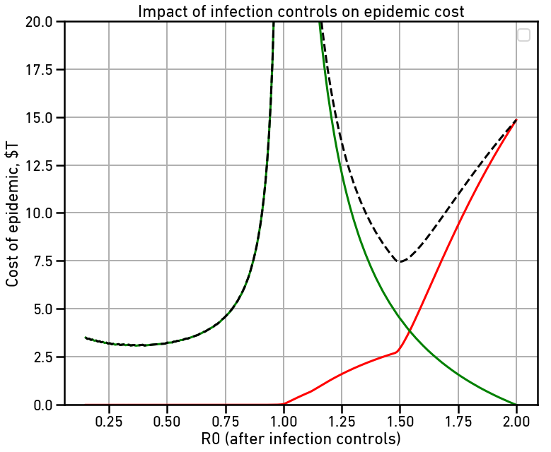
The red line is the cost of the disease itself, largely due to deaths. The green line is the cost of maintaining infection controls throughout the epidemic. The dashed line is the total cost, all in billions of dollars. Note that with no controls, our estimate of the total cost to the US is $14.8 trillion dollars, or about 2/3 of the total US GDP.

There are two local minima on the total cost curve. The first is right around R0=1.50. This makes the spread slow enough that hospital capacity is never overloaded, greatly reducing the number of deaths and thus the cost of the disease. This reduces total cost to $7.45 trillion dollars, just about half of what the uncontrolled cost would be. Note that even with this small amount of reduction, the majority of the cost is due to the controls rather than directly due to the disease.

The second local minima is at the far left, right around at R0=0.35, or about what the Chinese managed in Wuhan. This slows the spread of the disease so fast that we rapidly enter back into the much cheaper contact-tracing regime where wholesale lockdowns are no longer necessary. This reduces total cost to $3.11 trillion dollars, half again the cost with only moderate controls.

The cost savings with very serious controls imposed as soon as possible comes from two sources: First, lower disease burden in deaths, hospitalization, and lost productivity. Secondly, it’s cheaper to impose very serious controls because they need to be imposed for a much shorter period of time to control the disease.

A basic SIR model for the epidemic.

Total population 327 million, with a single initiating infection. 12 day course of disease, initial R0 of 3.5 (as per the stats from China that Steve linked.) Assume 5% of cases are critical, 2% of those critical cases die with ICU care, 5% with general hospital care, and 50% with no care. 90,000 available ICU beds and 900,000 available hospital beds.

Run this model through to completion and it sweeps through the population in about a year, infecting most everyone (less about 9 million who escape), killing 5.4 million.

Now, suppose we impose infection controls on day 80, right about when there’s 1000 deaths from this thing. And then we vary how strong those controls are: from 0.35 (what the Chinese managed) up to nothing at all.

Here we see how the # of deaths varies with the strength of our controls. If we impose Chinese-style controls, we get away with only 5K deaths, or 1000-fold fewer than without the controls. But the inflection point isn’t just at 1.0. In particular if we can get the R0 below about 1.5 that gets us down under 500K, or a 10-fold reduction. At 1.0 we get down to about 50K.

If we take the slope of this plot, we can see the marginal impact of better controls at each point, in terms of # of deaths saved:

Why the discontinuity at R0 of just below 1.5? Well, here’s the number of critical cases over time for several different scenarios. The vertical line is when we impose controls, the horizontal lines are ICU bed capacity and total hospital bed capacity. Right below an R0 of 1.5, we dip the # of critical cases low enough that we never exceed hospital capacity. The trick here though is that until you get R0 below 1.0 you’re still sweeping through most of the population, just more slowly, slowly enough that the hospitals can handle it. And that means that, for example, if you get R0 to exactly 1.0 you have to keep those infection controls in place for ~5 years or else you’ll be back up close to 5million dead again.

Appendix: code to generate this model.

from __future__ import division
import numpy as np
import matplotlib.pyplot as plt
from collections import namedtuple

PopState = namedtuple("PopState", [
    "day", 
    "susceptible", 
    "infected", 
    "dead", 
    "recovered",
])
EpiParams = namedtuple("EpiParams", [
    "days_infected", 
    "infection_rate", 
    "frac_critical", 
    "frac_dead_icu",
    "frac_dead_hospital",
    "frac_dead_home",
    "start_day",
    "controlled_infection_rate",
])

ICU_BEDS = 90000
HOSPITAL_BEDS = 900000

def update_state(state, params):
    day = state.day
    S = state.susceptible
    I = state.infected
    D = state.dead
    R = state.recovered
    N = S + I + D + R
    
    days_betw_contacts = params.days_infected / params.infection_rate
    if day >= params.start_day:
        days_betw_contacts = params.days_infected / params.controlled_infection_rate
    
    new_infections = (I * S) / (N * days_betw_contacts)
    recovered_infections = (I / params.days_infected) * (1 - params.frac_critical)

    # For critical cases, we split into ICU, hospital, and home care, in descending order
    C = I * params.frac_critical;
    C_icu = min(C, ICU_BEDS);
    C_hospital = 0 if C < ICU_BEDS else min(C - ICU_BEDS, HOSPITAL_BEDS)
    C_home = 0 if C < (ICU_BEDS + HOSPITAL_BEDS) else C - (ICU_BEDS + HOSPITAL_BEDS)

    recovered_critical = (
        ((C_icu / params.days_infected) * (1 - params.frac_dead_icu)) + 
        ((C_hospital / params.days_infected) * (1 - params.frac_dead_hospital)) + 
        ((C_home / params.days_infected) * (1 - params.frac_dead_home))
    )
    
    dead_critical = (
        ((C_icu / params.days_infected) * (params.frac_dead_icu)) + 
        ((C_hospital / params.days_infected) * (params.frac_dead_hospital)) + 
        ((C_home / params.days_infected) * (params.frac_dead_home))
    )
    
    newS = S - new_infections
    newI = I + new_infections - recovered_infections - recovered_critical - dead_critical
    newR = R + recovered_infections + recovered_critical
    newD = D + dead_critical
    
    return PopState(day + 1, newS, newI, newD, newR)

def run_model(state, params):
    infections = [state.infected]
    deaths = [state.dead]
    while (state.infected) >= 1:
        state = update_state(state, params)
        infections.append(state.infected)
        deaths.append(state.dead)
    return infections, deaths, state
	
total_population = 327 * 1e6
init_state = PopState(
    day=1,
    susceptible=total_population - 1, 
    infected=1, 
    dead=0, 
    recovered=0)
params = EpiParams(
    days_infected=12, 
    infection_rate=3.5, 
    frac_critical=0.05, 
    frac_dead_icu=0.02,
    frac_dead_hospital=0.05,
    frac_dead_home=0.5,
    start_day=79,
    # Modify this parameter to vary the strength of infection controls
    controlled_infection_rate=3.5,
)

infections_over_time, deaths_over_time, final_state = run_model(init_state, params)

Suppose we have a dominant mutation in the population with some prevalence . That means that a fraction of the alleles at that locus in the population are our mutation, while the rest are wild-type. We’d like to know how that prevalence changes over time. Some of those changes will be random, but we can average out to ask what the expectation of the change is at any particular point. We’ll have to make some assumptions first:

• Generations will be single events. We’ll start off with some generation, apply a selection model, and use that to generate the next generation, ad infinitum.
• Individuals will randomly mate to produce the next generation. This means there won’t be any population substructure and we can calculate the fraction of homozygotes and heterozygotes using only the mutation prevalence .
• The mutation confers a selective advantage that is equal in both homozygote and heterozygote carriers.

Given this, we can work out a table comparing different parts of the population, where is the probability of the wild-type allele:

	Wild-type	Heterozygote	Homozygote
Fraction of current generation
Relative fitness

Relative fitness here means that parents with the allele will have on average children if wild type parents have . That lets us calculate the fraction of the parents of the next generation, adjusting for increased reproduction of the carriers.

	Wild-type	Heterozygote	Homozygote
Relative proportion of parents
Normalized fraction of parents

Now that we know what fraction of the parental population has each status, we can calculate the expected prevalence of the allele after one generation. The next generation will have the same prevalence as in the parental population.

.

That is, we sum up half the fraction of heterozygotes and the fraction of homozygotes. This simplifies to

.

Note that for the case where , this reduces to , indicating no expected change in allele prevalence when there is no selective pressure, as we would expect. We can then calculate the change in prevalence as , which simplifies down to

.

This change is zero if and only if is zero. That is, if any of , , or are zero. This means that the allele changes frequency unless there is no selective pressure or the frequency is fixed at 0 or 1.

We can get a better handle on the behavior of this by treating it as a differential equation and solving. We can rewrite it as

.

Then we integrate both sides with respect to t:

.

Simplify the left side by partial fraction decomposition and solve the right side:

.

Then we simply integrate each piece of the left integral separately and combine the constants of integration.

.

There’s no way to solve explicitly for at any particular number of generations. Instead what this gives us is a solution for , the number of generations it takes to reach any particular prevalence, where the constant of integration is provided by the initial prevalence of the allele.

.

This lets us answer the question of how changes in the selection pressure affects the speed of selection. Suppose we keep the same starting prevalence and we wish to know how fast the population will reach some ending prevalence. The time needed is of the form

If then the time becomes approximately independent of . If then the time becomes approximately inversely proportional to the selection pressure. This gives us a bound on how fast increased selection can work: at most, doubling the selection pressure will half the time needed to increase allele prevalence to a given point.

Introduction

What happens to a new mutation?

Every person has some new mutations in their somatic genome, mostly caused by errors in DNA replication. They can pass that mutation on to their descendants. We know of a couple of historical mutations that look like they are all from a single common ancestor – for example, the common variant that’s responsible for blue eyes. How likely is a new mutation to succeed and become common?

This depends on the selective advantage of the new mutation. Relative to non-carriers, how many more surviving children do carriers of the mutation have than others? If non-carriers have on average child, then carriers will have children. Intuitively, higher selective advantage should make it more likely for a mutation to succeed.

We’re most interested in humans right now, and humans are diploid; they have two copies of each chromosome. Any variant can either be on both chromosomes or only one, and the selective advantage can be different depending on this. There are many common variants that are helpful when only one copy is present and harmful when two copies are present. Whether a mutation succeeds and becomes common mostly depends on the selective advantage in carriers with a single copy, because carriers with two copies are very rare when the mutation is uncommon.

There have been multiple approaches to solving this problem. Today we’ll look at one of the earliest and most simple. It’s straightforward, but requires a couple of assumptions that are not always valid. But we can get a lot of utility out of the simple result.

Haldane’s approach

Haldane’s original 1927 paper has a derivation of the likelihood of a new mutation becoming common, but it can be somewhat difficult to understand. We’ll work out his results in slightly more detail.

Suppose we have a large population with a new mutation present in a single individual. Let’s let be the chance that this mutation is passed down to of its children in the next generation. We’ll define a new function

We’ll see why this function is useful in more detail later. By construction, the coefficient of in is the probability of carriers in the next generation. Suppose instead we have multiple carriers in this generation. If the fraction of carriers is small, then we can ignore potential matings between carriers. That means that with carriers, the probability of carriers in the next generation is the coefficient of in .

Expanding on this a bit, suppose that and , so that each carrier has an equal probability of zero and one children who are also carriers. Then

If we have two carriers,

And we can see that the coefficients of the powers of x compose the probability distribution of carriers in the next generation.

Now, what would happen if instead of multiplying the function, we iteratively apply it to itself? This forms a composite function

Here the superscript denotes the number of times the function has been applied. Again, let’s look at this for our simple example. Applied twice,

We can see that this function represents the probability distribution of carriers after generations of reproduction. In this case, after each generation, half the carriers produce no children with carriers, so after two generations, we have only a 0.25 chance of a single carrier.

We can then represent the likelihood that the variant disappears from the population as . That is, as the number of generations goes up, what is the probability of no carriers in the population, represented as the coefficient of ?

This kind of repeated application of a function to an input is called a fixed point, and it will converge to a root of the equation if

1. is continuously differentiable around the fixed point.
2. .

Now, to be able to go further, we have to make some assumptions about the form of the function . We want to model the case of a new mutation with selective advantage , so that the expected number of carrier children of carriers with this allele is . We will model the probabilities as sampling from a Poisson distribution with mean , giving:

This can be simplified with some algebraic work I won’t show here to

So the probability of extinction is , where is the probability of survival, and we know that

So let’s plug into the fixed point equation , giving us

We take the natural log of both sides to get

.

Then we can take the Taylor series of to give us

Or simplify to give

.

Now, if the selective advantage is small, we can drop higher order terms, and we get Haldane’s result: the probability that the mutation survives from a single starting copy is .

Implications

First let’s remember the assumptions that went into this calculation:

• is “small”, so that we can drop higher-order terms in the Taylor series.
• The population size is “big”, so that we can ignore the likelihood of carrier-carrier matings.
• The number of surviving children per individual is Poisson-distributed.

The biggest implication of this result is that the likelihood of the mutation surviving doesn’t depend on the size of the population! It’s just as easy for a mutation to become common in a small population as a large population.

Second, the likelihood of survival is directly proportional to the selective advantage of the mutation. But since even highly adaptive mutations have low absolute values of , most new adaptive mutations are eventually lost.

Finally, if you repeatedly introduce the same beneficial mutation into a population, it’s very likely to become common. This suggests that even small amounts of crossbreeding will result in beneficial mutations from one population becoming common in the other population.